Contents

• Overview

• Quick Start

• Display

• Instructions

• Advanced 

• Discussion

• Design

Overview

Here is a demonstration of a basic perceptual control autonomous agent that adapts to its environment in order to achieve its goal. It does so by changing the way it perceives the world. The environment of the agent comprises a natural image.

The framework and model used here is an early step towards a perceptual control model of visual recognition and visual feature hierarchy development.

Quick Start

Click the Run checkbox.

The perceptual control agent, represented by a red cross-hair, will start moving through the image in the top-left.

Design

The (visual) environment of the agent is the grey-level values of one row in the image. These are displayed as the blue line in the bottom-left graph (the red line is the mean value). The gold line in that graph is the goal value (the reference) the agent wants to achieve.

When the pixel value is the same as the goal, then the agent will stop moving. However, as you can see the goal value (initially 200) is way above the blue line. So, the agent never perceives its goal and, so, never stops.

Now, click the Perception checkbox. This adds the magenta line which represents what is perceived by the agent, rather than the environmental inputs (the pixel values). The perception is the “weighted” input. Initially, these are the same as the weight value is 1.00.

Learning takes place automatically by adjusting (reorganising) the weight value until the goal is reached. Watch this happen by kicking off learning by checking the Learn checkbox.

You will see the perception change, even though the environment does not, until the perception matches the goal (+/- 1) and the agent stops.

You can speed things up a great deal by dragging the speed scrollbar to the right hand side.

If you would like to see learning continue, then uncheck the Goal box.

Display

The display items and controls are as follows:

The left column from the top.

Image

The image which is the environment of the agent. You can click in the image to change the environment to a different row. If you move the mouse over the image you can see displayed the pixel values by row and column.

Controls

Reference scrollbar – to change the goal value of the agent.

Image drop-down – select a different image as the visual environment.

The checkboxes:

• Run – stop and start the demo.
• Goal – toggle stopping when the goal is reached.
• Learn – toggles the reorganisation.
• Perception – toggles the display of the weighted input in the graph below.

Control System – the display of the values of the main control system loop; the reference, the perception, the error (difference between reference and perception) and the output (the image column).

Speed Scrollbar – the speed of the demo. The initial value is “normal” speed. Move the scrollbar to the right to run the demo up to 50 times faster.

Perceptual Input Graph

A plot that shows the environment of the agent, which is a row of the image. The red line is the mean of all the values in the row (actual value displayed below axis in blue). The gold line shows the reference goal of the agent, which is set by the reference scrollbar. The red cross-hair corresponds with the one in the image and indicates the position of the agent in the column.

If you click on the blue or magenta line you can see the value of the plot point.

Also shown is a green dot which is the ratio of the reference divided by the weight. Can you work out what value that ratio converges to, due to the process of reorganisation?

---

The right column from the top.

Error Graph

The global error response of the system plotted against the weight value. The global error is the sum (see advanced section) of errors experienced as the agent travels over an entire row. The weight is adjusted in order to minimise this error response. During the process of adaptation you will see this error reduce to zero.

Error Graph controls – below the error graph are displays that show the actual values of the error and weight plot values. Also, are two controls which determine the number of points in the plot; the default is 1000.

• NumPoints – allows you to set the number of points to retain to track the history of the error curve.
• Clear – this button enables you to empty the current points recorded, which would then build up again to the number defined by NumPoints.

Advanced Controls

The controls in the advanced section provides the ability to try out different methods for the reorganisation and the error response, as well as testing the behaviour of the reorganisation algorithm.

Reorganisation – a drop-down that allows you choose between one of three reorganisation algorithms. The purpose of the reorganisation algorithms is to determine the direction in which to change the weight parameter such that the change results in reducing error. This direction is defined by a value between -1 and +1 and determined by the reorganisation algorithm. A negative value means a bit is taken off the parameter; vice versa for positive.

• Ecoli – if the error response is not reducing then a new direction is taken by selecting a random number between -1 and +1.
• EcoliBinary – if the error response is not reducing then a new direction is taken by selecting a random number between -1 and +1.
• HillClimb – if the error response is not reducing then the direction, of +1 or -1, is reversed. In other words, if the error curve is going up hill the direction is changed to go down hill.

Error Response – the error response is the persistent error within the system rather than the error at one point of time within a particular control unit. It represents the history of the error, in this case over a period defined by one cycle of perceiving the environment; the number of columns in the image (400 iterations).

There are two methods implemented here:

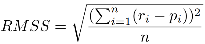
• RMSS – the square root of the mean of square of the sum of the unit error.

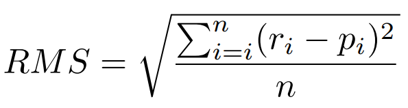
• RMS – the square root of the mean of sum of the squares of the unit error.

Weight – this drop-down box allows you to change the weight value manually to see how the reorganisation happens from different starting points.

Tumble – clicking this button will select a new direction of change. If one of the Ecoli algorithms is being used the direction will be random. For HillClimb it will flip the current direction.

Reset – the reset button halts processing and resets some of the demo settings.

Direction Graph

The final display component shows the direction of change of the parameter being adjusted. In this case the parameter is the weight of the environmental input, which gives the agent’s perception. The last 10 values are shown to see how it changes. Horizontal is zero and the maximum value of 1 is about 30 degrees off the horizontal.

The magnitude of the direction value indicates how much the weight will change. If the value is 0.05 then the weight will change relatively slowly compared to 1.00.

Instructions

In addition to the instructions given above, here are a few things to try out to see what happens to the learning behaviour. Try with the Goal box unchecked.

• Change the reference goal to see how the system adapts the way it perceives the environment.
• Click different rows in the image to change the visual environment of the agent. You can actually drag the mouse through the image and see the blue line change dynamically.
• Choose a different image entirely, from the drop-down box.
• Clear or change the number of points in the error plot to get a closer view of the error changing.

Did you work out what the green dot is doing? As a reminder the green dot is the ratio of the reference value over the weight. This ratio converges to the mean of the environmental inputs. As you can see it ends up on the red line, which is the mean. Try changing the reference to see the green dot move back to the red line. Likewise, with changing the row or the image see the green dot converge on the new mean.

So, the system has unintentionally “found” a property of the environment. There is nothing in the system design that explicitly tries to determine that value; it is a by-product of a closed-loop system controlling its perceptions and adapting to the environment.

Advanced

If you are interested in looking at this demo in more depth you can try out a few things related to the different types of reorganisation and the types of error response.

Each reorganisation algorithm selects a new direction if, at the end of each period, the error has not decreased.

The initial algorithm, Ecoli, randomly selects a number between -1 and +1, which defines the direction. This can mean that it may go in the wrong direction. However, that is only temporary as that would increase the error, and the system quickly corrects itself. Try this out by clicking the Tumble button when the error is on a descending slope until the sign of the direction is the opposite of what it was.

This image shows an example of this. Although the error reduction goes off track for a few cycles it quickly reverts to the right direction entirely by random selection.

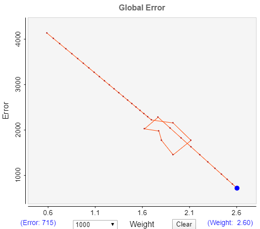
One drawback of the Ecoli algorithm in this current implementation is that the slope of the direction can be very shallow (close to zero) which means that the learning is very slow.

However, that is due to the periodic method of selection. In future demos we will try a method for accumulating the error which would mean that a shallow slope would result in a quicker change of direction.

The issue is partially resolved by the second algorithm, EcoliBinary, which limits the direction magnitude to 1 (not close to zero). It should also be noted that when the error is near zero a shallow slope can be useful to stay in the area of low error.

Try out the Tumble with the other two algorithms, EcoliBinary and HillClimb.

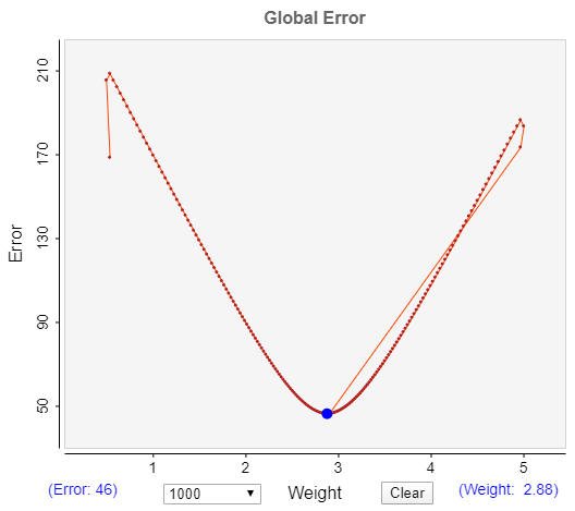
With the methods of error response you can explore the different error curves. Let the error reduce to around zero and then, with the Weight drop-down box, select a new weight that is on the opposite side of the current weight trajectory.

When the error returns to zero you will see the error curve. As these images show the RMSS error “curve” is v-shaped, whereas RMS is a curve. Also RMSS gives a better result for the weight value. In this example the reference is 250 and the mean is 83.79. So, for RMSS the ratio gives a mean of 83.61 whereas RMS gives 86.80. Additionally RMS does not converge to zero as RMSS does.

Discussion

This is a demonstration of a perceptual control system that adapts to its environment.

The system includes the constituent components of a perceptual control loop. Though these are quite basic, meaning the control is very limited.

The environment is quite erratic and discontinuous, as is the perception of the environment so is difficult to control. A comparator function derives an error signal, which is the difference between the reference goal and the perception. That error is used by an output function (a hard sigmoid) which determines whether the agent should move or not. That movement affects the agent’s position in the environment and, so, the perception, closing the loop.

Although the control is limited what the system does do is change the way it perceives the environment in order to realise its goal.

As these demos progress we expect the systems to be able to develop perceptions that are more sophisticated, high-level combinations of inputs, leading to much easier and smoother control.

Design Parameters

1D – the agent’s environment is one dimensional; one row through an image.

Single pixel – the perception of this agent is derived from just a single pixel at a time.

Proximal – the field of view of the agent consists of only the pixel at the agent’s current position. It cannot see pixels at any other position.

Adaptive – the structure of the control system adapts, by adjusting the input weight in such a way that the overall system error is minimised.

Binary – The output of the system is binary 1 or 0, based upon the presence or not of error. If there is error, then the agent moves 1 pixel to the right.